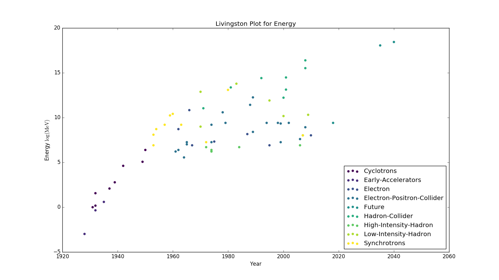
As part of the homework for a particle physics class I was required to make a few livingston plots. A livingston plot is similar to something you’d expect to see from a Moore’s law but for particle physics. Instead of plotting number of transistors on a log scale vs year though particle physicists will look at the log of the energy vs year.

Livingston plots:

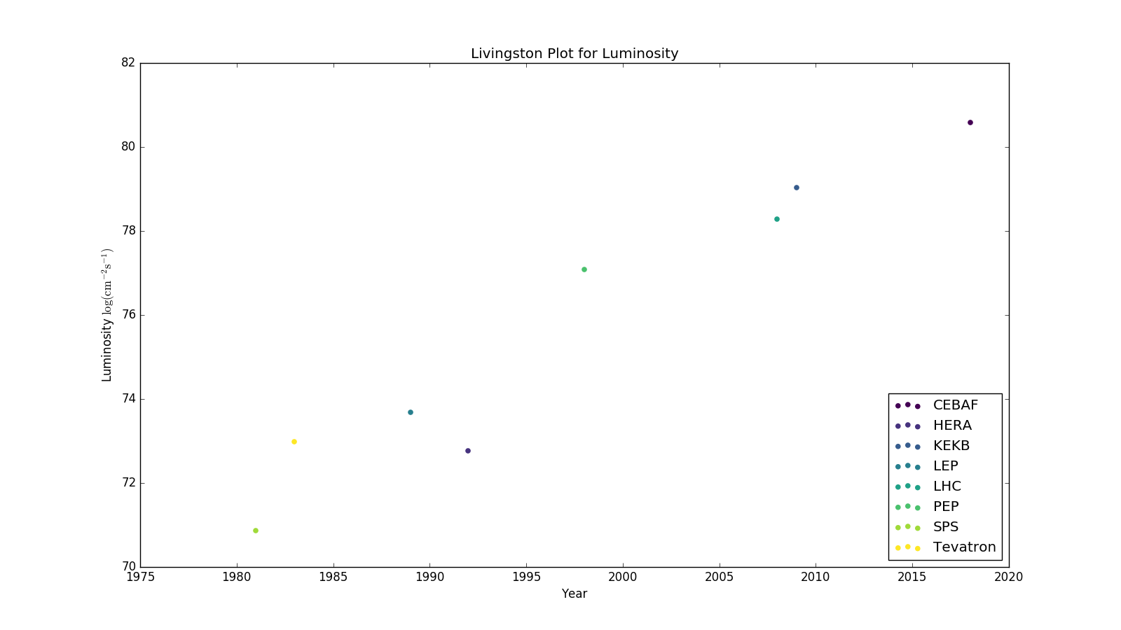
You can also look at the log of the lumunosity vs year. Luminosity can be a little difficult to understand but it’s easy to think of it as the brightness of the particle beam.

The full code and data can be found at my Homework github repository but I’ll share part of the code here. This section goes through and:

1. Opens json file
2. Creates a dataframe
3. Finds the unique types and assigns a color to them using a dict
4. Then for each type the data is added to the scatter plot

with open('acc.json') as data_file:
    data = json.load(data_file)

df_acc = pd.DataFrame(data["Accelerator"])
df_acc['logE'] = df_acc["Energy_MeV"].apply(np.log)
types_acc = np.hstack(np.array(df_acc['Type']))

uniq_acc = np.unique(types_acc)
values = cm.rainbow(np.linspace(0,1,len(uniq_acc)))
col = dict(zip(uniq_acc, values))

for i,acc in zip(xrange(len(uniq_acc)),uniq_acc):
    temp = df_acc[df_acc['Type'] == acc]
    year = np.hstack(np.array(temp['Year']))
    logE = np.hstack(np.array(temp['logE']))
    plt.scatter(year, logE, alpha=1,color=col[acc],label=r'%s' %(acc))

plt.show()

#First Post

The first post on my new site.

    def hi():
        return "Hello World!"